Setting Up A Reproducible Workflow in R

Starting a New Project

Every reproducible R workflow starts the same way: a version-controlled project with an isolated package environment. Getting both of these in place from the very beginning is much easier than retrofitting them later, and both Positron and RStudio make it straightforward.

Before walking through the steps for each IDE, there is one recommendation worth making upfront: always package your R code. I will talk more about this in the [INSERT CROSS-REFERENCE HERE] of this guide.

This might sound like overkill for a one-off analysis, but the structure that comes with an R package (a clean DESCRIPTION file, a defined namespace, a place for documentation and tests) pays off quickly as a project grows. The tradeoffs are minimal, and the habits it builds are good ones. The only naming constraint to be aware of is that R package names may only contain letters, numbers, and periods; they must start with a letter; and they cannot end in a period. No hyphens, no underscores.

If you need more information on how R Packages work, the best suggestion I can give you is to read the R Packages book written by Hadley Wickham and Jennifer Bryan. It may seem overwhelming at first, but after grasping how things work, you will come to understand that it is easier than what people expect.

Positron

1. Click on New (top left corner of the window) and select Create a New Folder from Template.

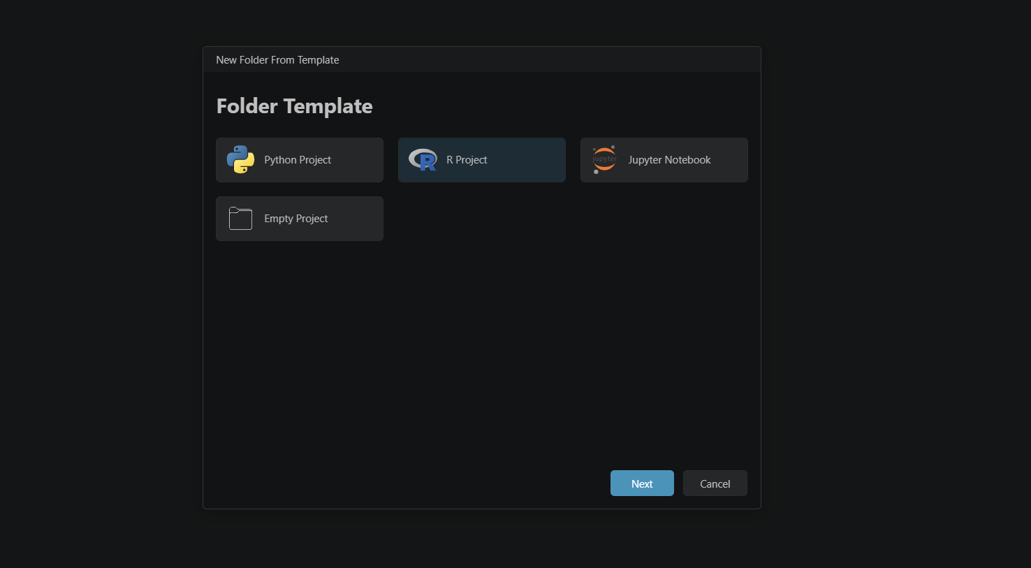
2. In the setup window, select R Project and click Next.
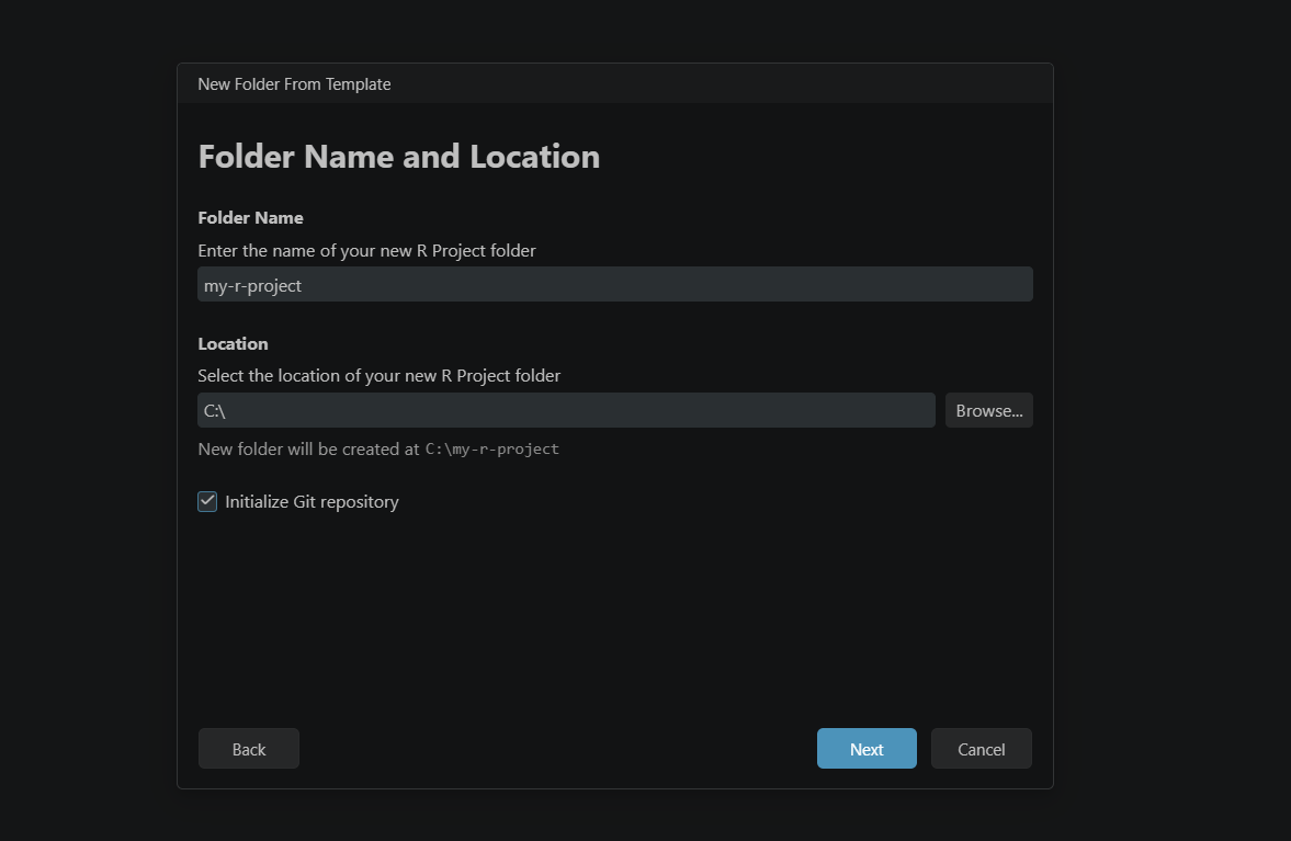
3. Enter a name for your project folder and choose where it will live on your machine. At this step, make sure to tick Initialize Git repository before continuing. Apply the naming rules above if you are following the packaging recommendation. Click Next.

4. Select the R version you want to use (if you have more than one installed). This is also where you tick Use renv to create a reproducible environment. Click Create.
5. Positron will ask where you want to open the new project. Either option works fine, but opening it in the current window keeps things tidy.
6. Once the session loads, give it a few seconds before continuing.
7. To set up your current R project to follow the structure of an R package, you need to run the following command in your R console:

usethis::create_package(getwd())

RStudio

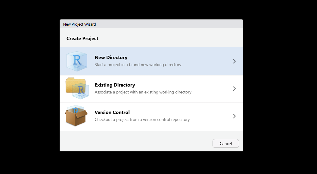
1. Go to File > New Project.
2. Select New Directory in the setup window.
3. Choose R Package if you are following the packaging recommendation, or New Project if not.

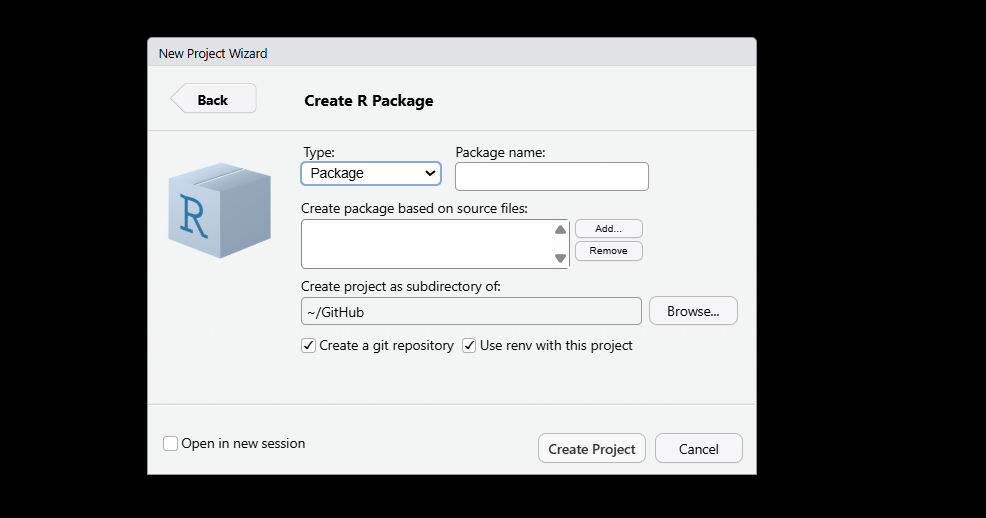
4. Enter your package (or project) name, applying the same naming rules as above. Before clicking Create, make sure to tick both Create a git repository and Use renv for this project.

---

Regardless of which IDE you used, you now have two of the most important foundations for a reproducible workflow in place: an isolated package environment managed by renv, and a Git repository ready to start recording the history of your project. Everything else builds on top of these two things.

Assuming that you selected the R Package structure, your directory will end up with an initial structure that looks something like this:

   ls -Force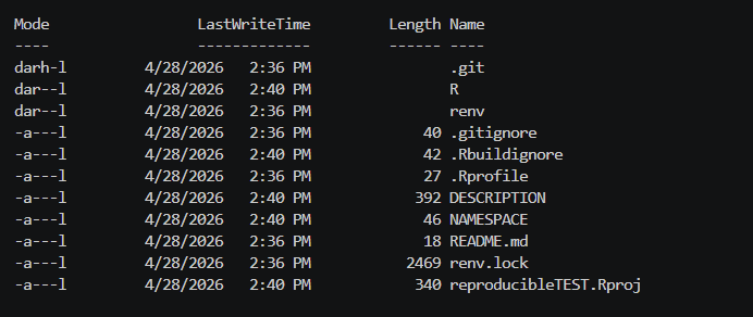

Version Control with Git and GitHub

With Git initialized in your project, you have a system that records every intentional change you make to your codebase. But having Git set up and actually using it well are two different things. This section covers the core commands you will reach for on a daily basis, explains what each one does, and closes with a habit that will serve you well long before you ever work on a team.

All of the commands below are run from your terminal, inside your project directory.

INFO

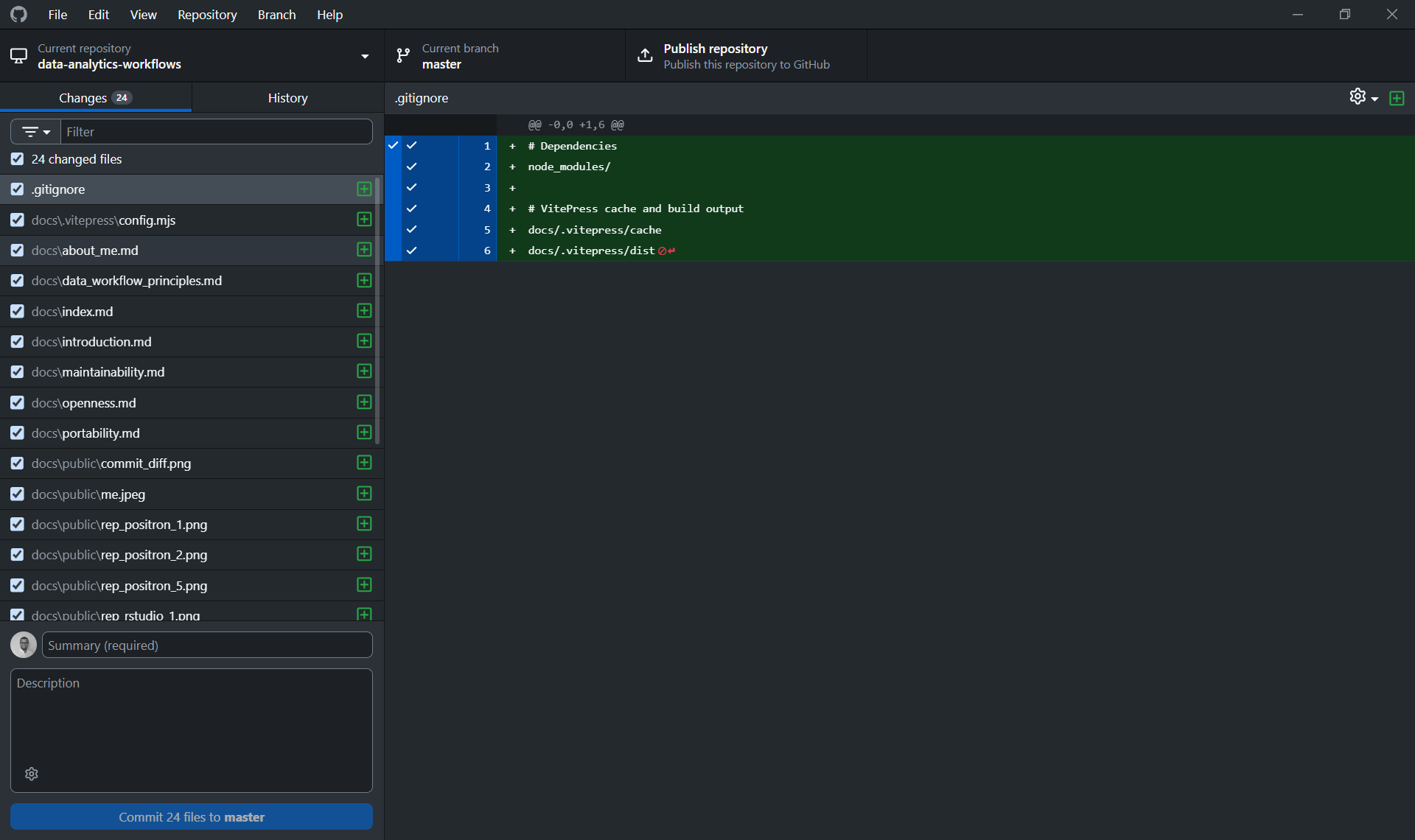
A note on GitHub Desktop

If you are new to Git and the terminal feels like too much at once, GitHub Desktop is a visual interface that lets you commit, push, pull, and manage branches without writing a single command. It is genuinely helpful for getting started and understanding what is happening visually before the mental model fully clicks.

That said, the recommendation here is to use it as a bridge, not a destination. The terminal commands are simple, universal, and available in every environment you will ever work in. A GUI is not. Getting comfortable with the commands above means you are never dependent on a specific tool, and you can work just as fluently on a remote server, a CI pipeline, or a colleague's machine as you can on your own.

Linking your local repository to GitHub

At this point, you have a local Git repository, but it only exists on your machine. To push your work to GitHub and make it accessible to collaborators (or just safely backed up), you need to create a remote repository and link the two together.

From the terminal, the process is two steps: first create an empty repository on github.com (with no README, .gitignore, or license, since your local project already has its own history and adding those files on the GitHub side will create a conflict), then link it to your local project:

# Link your local repo to the GitHub remote
git remote add origin https://github.com/your-username/your-repo-name.git

# Rename the default branch to main (if it isn't already)
git branch -M main

# Push your local history to GitHub and set the upstream tracking branch
git push -u origin main

The -u flag sets the upstream tracking relationship, meaning that from this point on, a plain git push or git pull will know which remote branch to talk to without you having to specify it every time.

From GitHub Desktop, this is simpler: clicking "Publish Repository" handles both steps at once, creating the remote repository on GitHub and linking it to your local project in a single action. This is one of the cases where the GUI genuinely saves you a step. That said, it is still worth knowing what is happening under the hood.

INFO

It is also worth knowing that both RStudio and Positron have native Git integration built directly into the IDE. You can stage files, write commit messages, push, pull, and manage branches without ever leaving your editor. If you prefer to keep everything in one place, that is a perfectly reasonable way to work. Personally, I find GitHub Desktop cleaner for this, since it keeps version control concerns separate from the coding environment, but this is genuinely a matter of taste. All three options, terminal, GitHub Desktop, and your IDE, are talking to the same underlying Git repository, so whatever feels most natural is the right choice.

After either approach, your local repository and GitHub are in sync, and you are ready to follow the branching workflow described below.

The core commands

Staging and committing changes

A commit is a named, timestamped snapshot of your project. Before you can commit, you need to tell Git which changes to include, this is called staging.

# Stage a specific file
git add path/to/file.R

# Stage all changed files in the project
git add .

# Create a commit with a descriptive message
git commit -m "Add data cleaning function for income variable"

A good commit message describes why the change was made, not just what file was touched. "Fix bug" tells you nothing six months from now. "Fix null handling in income variable before model fitting" does.

Pushing changes to GitHub

Once you have one or more commits locally, you push them to the remote repository on GitHub so they are backed up and visible to collaborators.

git push origin your-branch-name

Fetching and pulling changes from GitHub

When collaborators (or you, from another machine) have pushed changes to GitHub, you need to bring those changes into your local copy.

# Fetch checks what has changed on the remote, without applying anything yet
git fetch origin

# Pull fetches and immediately merges those changes into your current branch
git pull origin your-branch-name

A good habit is to always pull before you start working in a session, so you are not building on top of a stale version of the code.

Creating a new branch

A branch is an isolated copy of the codebase where you can work freely without affecting the main version. When the work is ready, it comes back through a pull request (more on that below).

# Create a new branch and switch to it immediately
git checkout -b feature/add-cleaning-functions

Branch names should be short and descriptive. Prefixes like feature/, fix/, or analysis/ help keep things organized as a project grows.

Opening a pull request

A pull request (PR) is a request to merge your branch back into the main branch. It creates a review checkpoint, a moment where the change is visible, discussable, and intentional, before it becomes part of the permanent record. Pull requests are opened through the GitHub web interface (or via the GitHub CLI), not from the terminal directly.

Once you have pushed your branch:

git push origin feature/add-cleaning-functions

Go to your repository on GitHub. You will see a prompt to open a pull request for your recently pushed branch. From there, add a description of what changed and why, and merge it when it is ready.

Always work on a branch, even alone

It might feel unnecessary to create a branch when you are the only person on a project. It is not. The habit of never committing directly to main is one of those things that costs almost nothing to practice alone and pays off immediately the first time you collaborate with someone else. Beyond collaboration, branches let you keep the main version of your code in a working state while you experiment, and they give you a clean place to abandon an approach that did not work out without leaving traces in the main history.

Make it a rule: new feature, new analysis, new idea, new branch.

Managing Dependencies with renv

When you initialized your project with renv, it created an isolated package library specific to your project and a file called renv.lock. This lockfile is the heart of reproducibility on the dependency side: it records the exact version of every package your project depends on, along with where it was installed from (CRAN, GitHub, Bioconductor, etc.). When someone else clones your repository and restores the environment, they get exactly the same packages you had, not just the same names, but the same versions.

The renv.lock file should always be committed to version control. It is what makes the "clone and run" promise actually work.

Installing packages

Rather than using install.packages() directly, install packages through renv:

renv::install("dplyr")
renv::install("tidyr")

# Install from GitHub
renv::install("tidyverse/dplyr")

This ensures the package is installed into your project's isolated library rather than your global R environment.

Snapshotting your dependencies

Here is something that trips people up at first: installing a package does not automatically write it to the lockfile. You have to explicitly take a snapshot of your current environment for renv to register the change.

renv::snapshot()

But there is a subtlety here worth understanding. renv::snapshot() does not blindly record every package installed in your project library. It only records packages that are actually used in your project, meaning packages that appear in a library() or require() call, or are referenced directly via :: (like dplyr::filter()) somewhere in your code. If you install a package but never reference it in a script, renv will not include it in the lockfile. This is a feature, not a bug: it keeps the lockfile lean and honest about what your project truly depends on.

The practical habit to build is: install a package, use it in your code, then run renv::snapshot() before committing.

Checking the status of your environment

At any point, you can check whether your project library, your lockfile, and your actual code are all in agreement:

renv::status()

This will tell you if there are packages that are installed but not yet snapshotted, packages in the lockfile that are no longer used, or any other drift between what the lockfile says and what is actually in your environment. Running this before committing is a good habit, the same way you would check git status before staging files.

Restoring an environment from the lockfile

When you clone a repository that uses renv, or when a collaborator shares their project with you, the first thing to do is restore the environment:

renv::restore()

This reads the renv.lock file and installs every package at the exact version recorded there. Once it finishes, you are working in the same environment as whoever created the lockfile, regardless of what you have installed globally on your machine.

Versioning Data with pins

For data versioning in R, there are two solid options worth knowing about: DVC and pins. DVC is a powerful tool that ties data versions directly to your Git history, and we will cover it in detail in the Python workflow guide, where it feels more at home. For R, pins is the more natural choice. It fits comfortably within the Posit ecosystem, the API is clean and straightforward, and the mental model maps well onto how most R users already think about sharing and retrieving data.

The core concept in pins is a board: a storage backend where you publish and retrieve versioned artifacts. Boards can be local folders, network drives, Amazon S3 buckets, Google Cloud Storage, Azure storage, or Posit Connect. The same workflow applies regardless of which backend you use, and you can switch backends without changing the code that reads and writes your data.

Setting up a board

There are three board options you will reach for most often, depending on your setup.

board_folder() stores pins in a specific folder you point it to. This is the most explicit and portable option for local work, and the one I would recommend as a starting point. You can point it at a folder inside your project, or at a shared network drive if your team works from one:

library(pins)

# Store pins in a local folder within your project
board <- board_folder("data/pins")

# Or point to a shared network drive
board <- board_folder("//network/shared/project-data")

board_local() stores pins in a user-level cache directory that persists across all projects on your machine. This is useful when you want to share a dataset between different local projects without duplicating files, but it is less explicit about where things live and not portable to other machines:

board <- board_local()

board_s3() is the natural step up when you are working in a team and need a shared backend that everyone can access regardless of their machine. Any collaborator with access to the bucket can read and write pins using the same code:

board <- board_s3("your-bucket-name")

For solo work or early project stages, board_folder() is the right default: zero infrastructure overhead, explicit about where your data lives, and easy to commit the folder path to your project documentation. Switching to board_s3() later requires changing only one line of code.

Writing and reading pins

Publishing a dataset to a board is done with pin_write():

board |> pin_write(clean_survey_data, "clean-survey-data", type = "parquet")

The type argument controls the file format. Parquet is the recommended default for tabular data: it handles column types explicitly, compresses well, and reads efficiently. Other options include "csv", "rds", and "json".

Retrieving a pin later is equally straightforward:

df <- board |> pin_read("clean-survey-data")

How versioning works

Every time you call pin_write() on an existing pin, pins does not overwrite the previous version. Instead, it creates a new timestamped version alongside the old one. Each version gets a unique identifier, a hash, a file size, and a creation timestamp. This means you always have a full history of how a dataset has changed over time, and you can retrieve any specific version if you need to.

To see all available versions of a pin:

board |> pin_versions("clean-survey-data")

To retrieve a specific version rather than the latest:

board |> pin_read("clean-survey-data", version = "the-version-id")

Logging pin metadata alongside your outputs

Where pins really earns its place in a reproducible workflow is when you log exactly which version of a dataset was used to produce a given output. Every pin comes with metadata you can retrieve and store as part of your runtime record:

meta <- board |> pin_meta("clean-survey-data")

metadata <- list(
  timestamp = Sys.time(),
  input = list(
    name = meta$name,
    version = meta$version,
    hash = meta$hash
  )
)

Saving this alongside your outputs closes the traceability loop: anyone looking at a result can see not just which code produced it, but exactly which version of the data was used.

Best Practices for Managing Your Project as a Package

Structuring your project as an R package is not just about following conventions for their own sake. It gives you a framework that enforces good habits around dependency management, code organization, and separation of concerns. Here are the practices worth building into your workflow from day one.

Storing secrets with edit_r_environ()

As covered in the portability section, secrets and credentials should never appear in your code or in any file committed to version control. In R, the standard place for these is your .Renviron file. The easiest way to open and edit it is through usethis:

usethis::edit_r_environ(scope = "project")

Using scope = "project" creates a project-level .Renviron file rather than editing your global one, which keeps your secrets scoped to the project and avoids accidentally exposing them across other work. Add your credentials in that specific .Renviron file:

API_KEY="your-api-key-here"
DB_PASSWORD="your-db-password-here"

Make sure .Renviron is listed in your .gitignore. Then reference the variables in your code using Sys.getenv():

api_key <- Sys.getenv("API_KEY")

Recording dependencies in the DESCRIPTION file

When you use renv, your lockfile tracks the packages installed in your project library. But when your project is structured as a package, there is a second place where dependencies need to be recorded: the DESCRIPTION file. This is what tells R (and anyone installing your package) which packages it formally depends on.

Every time you start using a new package in your project, register it with:

usethis::use_package("dplyr")
usethis::use_package("ggplot2")

This adds the package to the Imports field of your DESCRIPTION file. Think of renv.lock as the precise, version-pinned record of your environment, and DESCRIPTION as the human-readable declaration of what your project needs. Both serve a purpose and both should be kept up to date.

Organizing your code: the R/ folder and the scripts/ folder

R is a functional programming language, and the package structure encourages you to lean into that. The convention is worth following deliberately:

The R/ folder is where your reusable functions live. These are the building blocks of your workflow: cleaned, refactored, and general enough to be called from multiple places. Each function should do one thing well. This is also where R will look when loading your package, so anything in here becomes part of your project's defined interface.

# R/clean_data.R
clean_survey_data <- function(df) {
  df |>
    dplyr::filter(!is.na(income)) |>
    dplyr::mutate(income = as.numeric(income))
}

The scripts/ folder (or whatever name feels natural to you) is where your execution scripts live. These are the files that actually run the analysis: they call the functions defined in R/, load data, and produce outputs. The key discipline here is keeping these scripts short and linear. A script in this folder should read almost like a table of contents for what the analysis does, not like a place where logic is defined.

# scripts/01_clean_data.R
pkgload::load_all()

raw_data <- readr::read_parquet("data/raw/survey.parquet")
clean_data <- clean_survey_data(raw_data)
readr::write_parquet(clean_data, "data/processed/survey_clean.parquet")

This separation also directly addresses the linear execution and notebook trap we discussed in the traceability section. Scripts in scripts/ should always run correctly from top to bottom in a clean session. The logic lives in R/, the execution lives in scripts/, and the two never get tangled up.

---

Packaging your code unlocks a number of other good practices worth knowing about: documenting your functions with roxygen2 comments, managing raw data objects with usethis::use_data_raw(), and building a proper R/data.R to document datasets. These practices connect more closely to the readability and optimality principles, so we will come back to them later in the guide.